Explore the Scientific R&D Platform

Try Now
Pricing
MENU
Try Now
Pricing

Sample Size Determination Example

AREA: Andersen-Gill, Recurrent Events | Immunology

nQuery In Use Background Web  Opacity 35
Andersen-Gill (Recurrent Events) Worked Examples

Title: Sample size calculation for the Andersen-Gill model comparing rates of recurrent events

Objective: CGD is a rare immune system disorder characterized by recurrent pyogenic infections. Suppose we want to design a new trial to assess the effect of a new experimental product on the infection rate. (Example 1).

Year: 2019

Source: Statistics in Medicine

Link: https://onlinelibrary.wiley.com/doi/abs/10.1002/sim.8335

Clinical Area: Immunology

Sample Size Section in Paper/Protocol:

Suppose we want to design a new trial to assess the effect of a new experimental
product on the infection rate. We assume that the event rate function is of Weibull form
λ 0 (t) = ψνt ν−1 in the placebo arm, and the event rate ratio between the two treatments is
constant λ 1 (t)∕λ 0 (t) = exp(β) = 0.6 over time. We get the MLE (ψ, ν, κ)=(1.097 1.221 , 1.221,
0.871) by fitting an NB process model to the data using the SAS NLMIXED procedure on
basis of the likelihood function given in Equation (20) of Dean and Balshaw. Matsui
obtained similar point estimates based on the generalized estimating equations (GEE)
for the MPP

To determine the sample size, we assume a common dispersion parameter and
identical dropout pattern in the two groups. We set ψ = 1.1, ν = 1.2, κ = 0.8, which are
close to the MLE. The treatment allocation ratio is p1 ∶ p0 = 1 ∶ 1 or 2 ∶ 1. Both design 1
(planned treatment duration τc = 1 year for all patients) and design 2 (accrual period τa
= 0.5 year, additional treatment duration τc = 1 year, constant enrollment rate η = 0) are
considered. In both designs, the loss to follow-up distribution is exponential with mean
1∕δ = 4 years.

The sample sizes for these designs are as follows:
Design 1 Balanced: 365, Design 1 Unbalanced (2:1): 390
Design 2 Balanced: 335, Design 2 Unbalanced (2:1): 360


Summary of Necessary Parameter Estimates for Sample Size Calculation:

 Parameter Value
Significance Level (2-Sided) 0.1
Weibull Scale 1.1
Weibull Shape 1.2
Event Rate Ratio 0.6
Dispersion Parameter (both groups) 0.8
Exponential Dropout Rate 0.25
Power 90
Minimum Treatment Period 1
Accrual Period (Design 1;Design 2) 0;0.5 (enrollment = 0)
Sample Size Allocation (balanced/unbalanced) 0.5;0.333 (1:1;1:2) 


Email me this example in PDF format

Step 1:
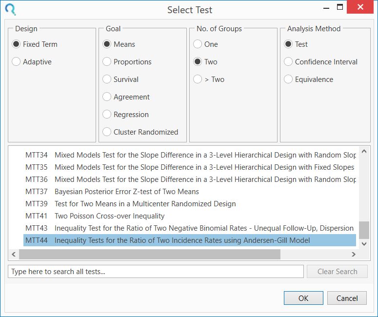
Select the MTT44 Inequality Tests for the Ratio of Two Incidence Rates using Andersen-Gill Model table from the Select Test window.

This can be done using the radio buttons below or alternatively, you can use the search bar at the end of the Select Test window and search for terms such as “MTT44” or “Andersen” and select the correct table.

After selecting the table in the window below the radio buttons, select OK to open the
table.

Andersen-Gill - Recurrent Events - Sample Size Example_Page_4_Image_0001

Step 2:
To replicate this example, the first four columns will be used for the balanced and unbalanced (1:2 controls:treatment) versions of Design 1 (no accrual period) and 2 (6 month accrual period).

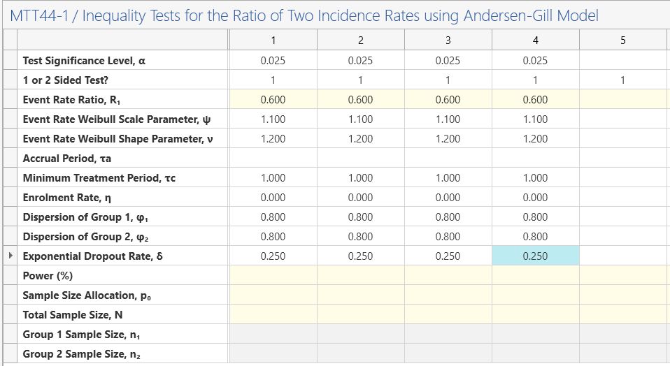
The following parameters are the same in each column:

Enter the significance level of 0.025 and select a 1-sided analysis.

Enter the event rate ratio of 0.6, the Weibull Scale parameter of 1.1 and the Weibull Shape
parameter of 1.2.

As the minimum treatment period is the same for each design, enter 1 in the minimum treatment row in each column. As the enrollment rate will be ignored for the case where accrual equals zero, set this value to 0 (uniform accrual) in each column.

Enter the group 1 and 2 dispersion as 0.8 as these are assumed to be the same in each group in the study design. Enter 0.25 for the exponential dropout rate. Note this is equivalent to the δ in the design above, where 1/δ = 4 years (equivalent to 21% dropout per year).

Andersen-Gill - Recurrent Events - Sample Size Example_Page_5_Image_0001

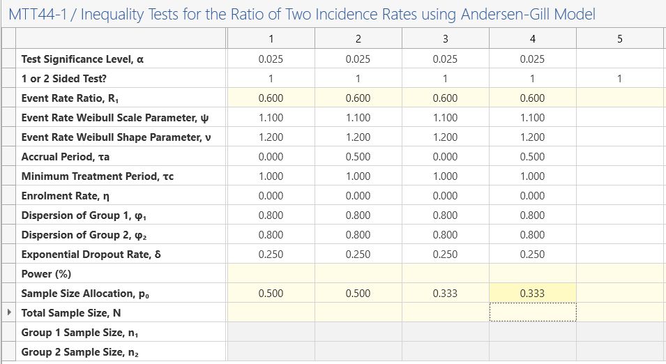
The balanced design 1, balanced design 2, unbalanced design 1 and unbalanced design 2 will be entered into columns 1-4 respectively.

In columns 1 and 3, enter an accrual period of zero. In columns 2 and 4, enter an accrual period of 0.5.

In columns 1 and 2, enter a sample size allocation of 0.5. In columns 3 and 4, enter a sample size allocation of 0.33333333.

Andersen-Gill - Recurrent Events - Sample Size Example_Page_6_Image_0001

Step 3:
Enter the power of 90% in each column and the Total Sample Size and per group sample sizes will be calculated.

Andersen-Gill - Recurrent Events - Sample Size Example_Page_7_Image_0001

Result:

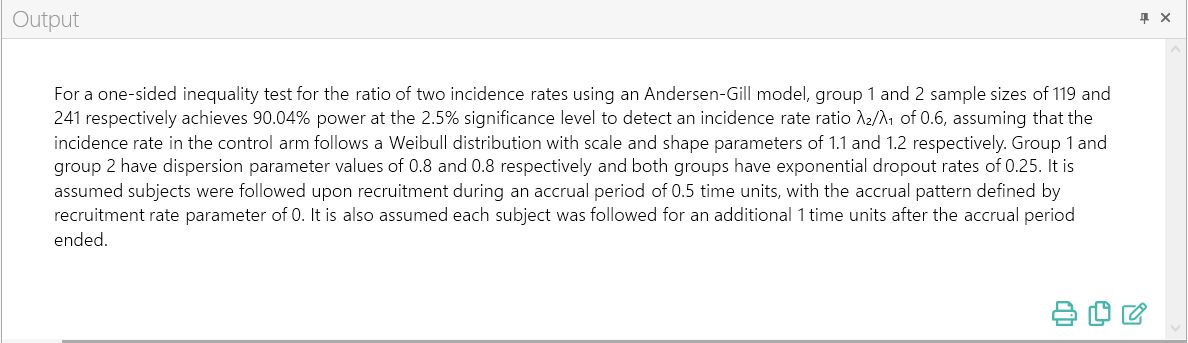
The analysis results in a sample sizes of 365, 335, 390 and 360 as per Table 1 in the paper.


We can summarize our results by using the output statement.

Andersen-Gill - Recurrent Events - Sample Size Example_Page_7_Image_0002

Email me this example in PDF format

Free 14 Day Trial

Demo Icon white
No download required