

Scientific intelligence platform for AI-powered data management and workflow automation


Scientific intelligence platform for AI-powered data management and workflow automation

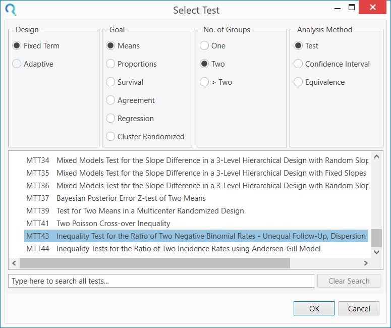
Step 1:
Select the MTT43 Inequality Test for the Ratio of Two Negative Binomial Rates - Unequal Follow-Up, Dispersion table from the Select Test window.
This can be done using the radio buttons below or alternatively, you can use the search bar at the end of the Select Test window and search for terms such as “MTT43” or “Negative Binomial” and select the correct table. After selecting the table in the window below the radio buttons, select OK to open the table.
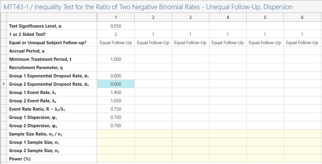
Step 2:
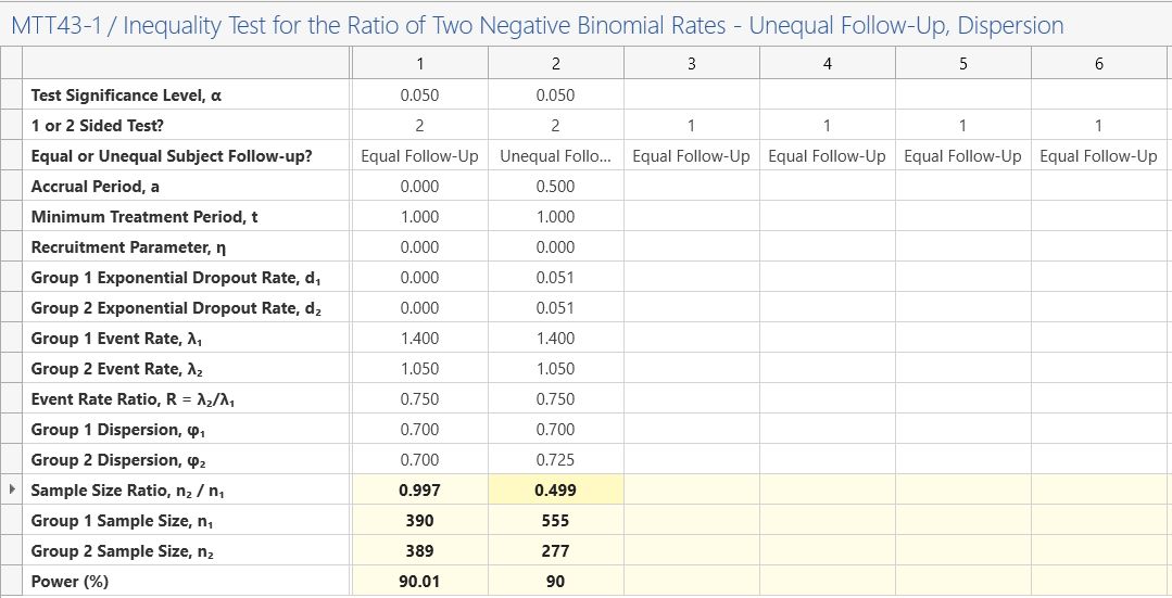
Enter the significance level of 0.05 and select a 2-sided analysis.
Then select “Equal Follow-up” from the third row and enter a minimum treatment period of one, for one year follow-up as per study design.
The accrual period and recruitment parameter rows can be set to zero as these are not needed for the equal follow-up scenario.
Enter zero for the group 1 and group 2 exponential dropout rates as dropout was not included in this calculation.
Enter the group 1 event rate of 1.4 and the event rate ratio of 0.75. This will automatically calculate the group 2 event rate of 1.05.
Enter the group 1 and 2 dispersion as 0.7 as these are assumed to be the same in each group in the study design.
Enter the a sample size ratio of one (equal sample size per group) and the power and the group 1 and 2 sample sizes will automatically calculate.
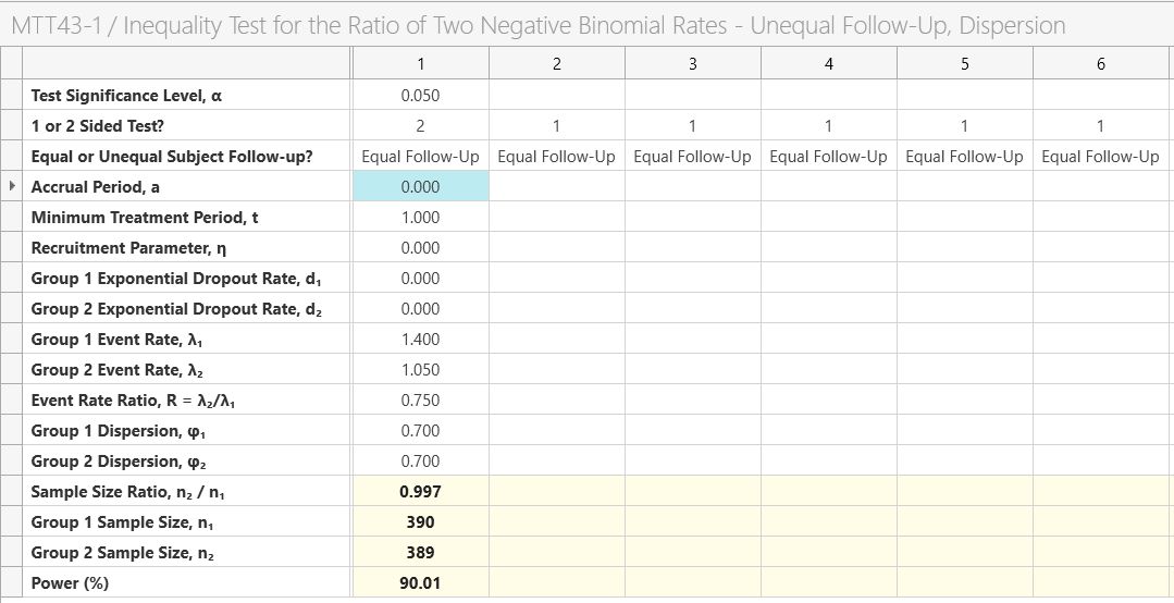
The analysis results in a sample size per group of 390 per group as per the study design. Note that group two is set to 389 for the exact power but to keep the sample size ratio exactly equal to one we would set both to 390.
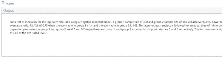
We can summarize our results by using the output statement.
In this table, there is the option to include the effect of unequal follow-up, dropout, unequal dispersion per group and unequal sample size.
To explore the effect of these on the study we will modify the above study to one with a study length of one and a half years but with uniform accrual over the first 6 months (½ year) of the study, a dropout rate per year of 5%, a higher dispersion of 0.725 in the treatment group and a sample size ratio of 2:1 for group 1:group 2.
To introduce these modifications, keep the values from the example above but change the third row to “Unequal follow-up”, set the accrual period to 0.5 (6 months = 0.5 years, note that total study time equals the accrual period plus the minimum treatment period), the recruitment parameter to zero (uniform accrual), the two exponential dropout rates equal to 0.0513 (see below for conversion), the group 2 dispersion to 0.725 and the sample size ratio to 0.5 (½).
| Result: |
|
This would give a total sample size of 555 + 277 = 782, |
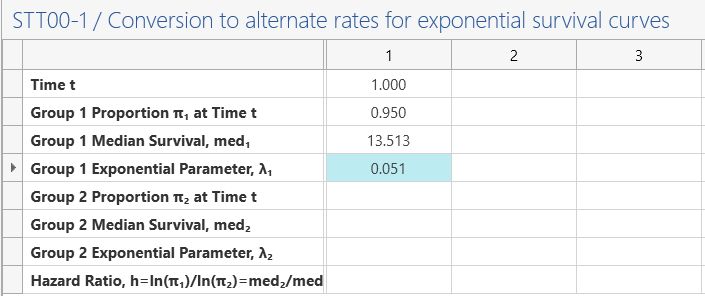
To calculate the exponential dropout, select “Survival Parameter Converter” from the Assistants menu.
Enter 1 in the Time row and 0.95 Group 1 (surviving) proportion. Then copy-paste the value in
the group 1 exponential parameter value.
|
This study can be expanded to demonstrate a Group Sequential design -Continue to see an example of this- |
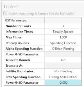
Suppose two interim analyses were planned after enrollments of one third and two thirds of the sample size. We will use an O’Brien-Fleming spending function to define the efficacy bounds and a non-binding Hwang-Shih-DeCani spending function with gamma parameter of -2 to define the futility bound.
The gamma parameter for the Hwang-Shih-DeCani gamma parameter would be a compromise between the conservative O’Brien-Fleming and liberal Pocock spending functions.
A non-binding futility boundary means we can cross the futility boundary and still continue the study without affecting the Type I error and is thus recommended in clinical trial design over binding boundaries.
| Parameter | Value |
| Number of Looks | 3 (equally spaced) |
| Alpha Spending Function | O’Brien-Fleming |
| Futility Boundary | Non-Binding |
| Beta Spending Function | HSD (Gamma= -2) |
Step 1:
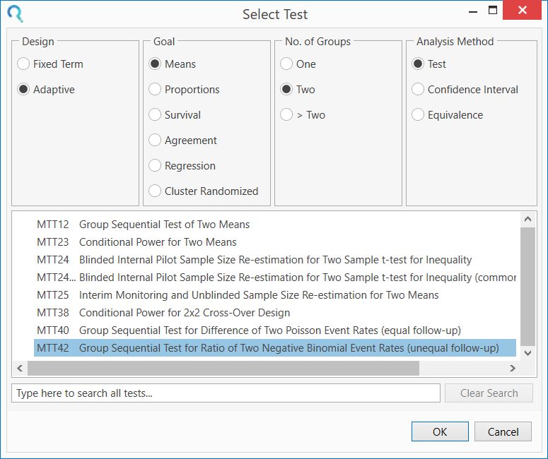
Select the MTT42 Group Sequential Test for Ratio of Two Negative Binomial Event Rates (unequal follow-up) table from the Select Test window.
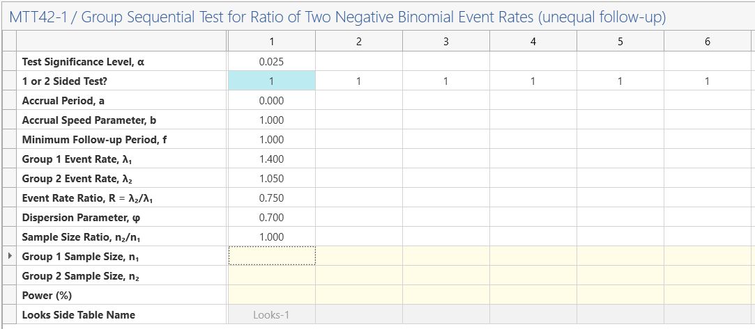
Step 2: As per the previous example, enter an accrual period of 0, an accrual speed parameter of 1 (note the speed parameter is ignored as the accrual period is zero i.e. equal follow-up per subject), a minimum follow-up period of 1, group 1 event rate of 1.4 and event rate ratio of 0.75 (group 2 event rate of 1.05 will automatically calculate), dispersion parameter of 0.7 and a sample size ratio of 1.
In this example, we will set the significance level as 0.025 (0.05/2) and a 1-sided analysis. These are equivalent analyses but allow for a meaningful futility bound which stops the trial early for event rate ratios which are too large (e.g. where new treatment is worse than control treatment).
Step 2: Enter the group sequential planning parameters above in the “GST Parameters” table in the side-table which appears automatically below the main table.
Step 3: Enter the power and the sample size and looks-side table will be completed.
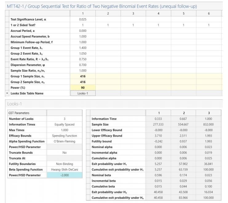
The GST design results in a sample size per group of 416 (compared to 390 for the fixed term
design).
The Looks table on the right-hand side of the side-table provides the bounds on the
standardized Z scale and the p-values required from a fixed term statistical analysis to stop early for efficacy (values less than nominal alpha at each look i.e. column) or futility (values greater than nominal beta at each look)
The output statement provides the following summary:
| Result: |
|
Sample sizes of 416 in group 1 and 416 in group 2 are required to achieve 90% power to detect an event rate ratio of 0.75 (assuming a group 1 event rate of 1.4 and group 2 event rate of 1.05) when there is a accrual period of 0 with an accrual speed of 1 and minimum follow-up of 1 using a one-sided test based on the Negative binomial model at the 2.5% significance level. These results assume that the group sequential design has 2 interim sequential tests (3 total looks including final analysis). The O'Brien-Fleming spending function is used to determine the efficacy test boundary. The Hwang-Shih-DeCani spending function (associated parameter -2) is used to determine the non-binding futility boundary. The drift parameter for this design equals 3.351. The drift parameter defines the increase in sample size needed over a fixed term design and equals square root of the maximum information level by the difference. |
